Practical example: Conjoint Analysis
Objective
A truck manufacturer wished to optimize his product line in the heavy truck (18 to 41 t) segment. With this in mind, equipment features were to be tested for acceptance among the target group, and the price acceptance for these features was to be investigated.
The aim was to forecast – taking into account external values such as market volumes and the costs of product features and services – which price positions for which product variants would lead to maximum profitability.
Analysis
To answer the above-mentioned questions, a conjoint analysis was conducted. In order to be able to make robust projections of concrete sales figures, a model was designed comprising the manufacturer’s brand alongside the four most important competitor brands. Additionally it included the following product features: cab, engine power, air conditioning, wind deflectors, paint, equipment version, various service packages and price.
164 decision-makers in companies using at least one truck in the relevant weight category were interviewed for the survey. In addition to a Choice Based Conjoint module, questions were also asked about, among other things, buying frequency and length of use. These were used to calculate weightings that were integrated into the forecasting model.
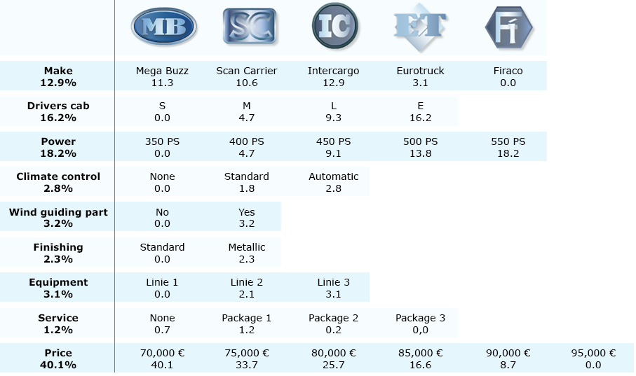
Fig. 1: Utility values of decision-makers in the heavy truck market
Hierarchical Bayes calculations based on the responses to the conjoint delivered individual utility values for each case. These represented the preferences of the respondents with regard to their requirements for a truck.
The required sales and profit projections were made with the aid of simulations. For this purpose, a project was set up in the online simulation tool MASIM into which the utility values and case weightings were integrated. Further, detailed production costs and market volumes were introduced into the model.
Firstly, a starting situation was defined which broadly corresponded to the existing market situation. A simulation of this constellation produced market shares that roughly approximated the real market, but with more or less major deviations from the actual market shares for all of the defined products.
Since the scenarios under investigation were meant to be oriented to the real market situation, adjustments were needed. The coefficients from the computer model were initially modified with the aid of optimization procedures so that the results of the simulation came close to the target figures without interfering with the data or making further case re-weightings. In a second and third adjustment step, the utility values were then adjusted for non-purchasers and manufacturers. With these steps, a perfect adjustment of the market model to the real situation was achieved.
Simulations based on this delivered cost-benefit relationships for the product features of interest. Thus it was possible to show the amount of additional value that individual extra items of equipment, product improvements or feature packages were worth to the respondents.
A simulation incorporating production costs and sales volumes was designed to show which product variants and which price positions could be expected to generate the maximum profit. For this purpose, fictitious products were constructed (a standard and a premium variant), which varied in certain features. The standard variant with its basic features had a lower price range than the premium variant with its more costly features. These variations generated 9,600 possible combinations. From these, MASIM calculated the most profitable combinations with the aid of its integrated optimization function. The following Figures show the result of this optimization.
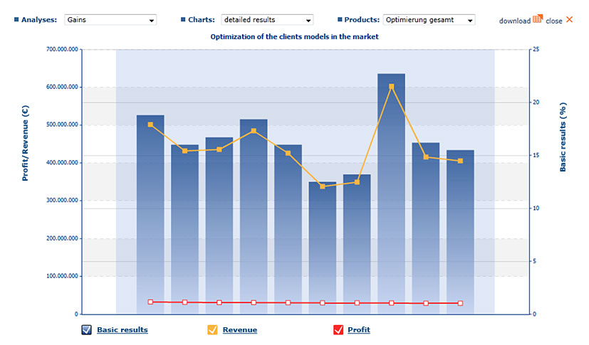
Fig. 2: Projected market shares, income and profit for the 10 combinations with maximum profit prospects
The red line in Figure 2 shows the projected profits for the 10 combinations with the highest profit expectations. As well as the profit curve, the Figure also shows expected market shares and incomes. The resulting scale range shows little differentiation with regard to profits. However it shows that, in contrast to profits, the calculated market shares and incomes vary significantly. Inclusion of these values can provide additional input to support decision-making. With combination 8, for example, not only high profits but also a strong market position is anticipated, because this has the highest projected sales volume.
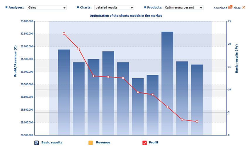
Fig. 3: Projected market shares and profit for the 10 combinations with maximum profit prospects
Figure 3 shows the results of the same optimization process, but excluding income. Now, the range of values can be scaled in such a way that differentiations in profit are made clear. This presentation makes clear that a combination of models exists which can lead to a very significant maximum profit.